Published on 30 Jun 2020 in Control Neural-Networks Predictive-Control Python Neurolab

Neural Generalized Predictive Control

In this post, I show how to do a simple Neural Generalized Predictive Control (NGPC) using Neurolab in python, To do this post I’m basing in the paper Neural Generalized Predictive Control A Newton-Raphson Implementation of Donald Soloway and Pamela J. Haley . If you want to know more about of state of the art of this techniques you can read the paper. In this post only show a bit of theory and the implementation of the simulation. All the training and simulation is made with Python using neurolab, numpy, matplotlib, random and scipy packages.

Neural Generalized Predictive Control

The NGPC is based in a Model Predictive Control (MPC) the difference is that the NGPC use a Artificial Neural Network (ANN) to do the prediction of the system. An ANN predict the next state of the system, with this prediction calculate the control input $u(t)$ to follow a reference $Ref(t)$ . The control input calculated based in a cost function $J$ and used a algorithm to minimization. A block diagram of NGPC is

Diagram-of-control

ANN to predict

The architecture of the network is like show the next image

Diagram-of-ANN

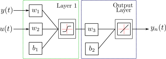
The input layer have to inputs, the input of the system $u(t)$ and the actual system state $y(t)$ . For this layer need to find the weights $w_1$ , $w_2$ and the bias $b_1$ . The activation function is a $tanh()$ . For the output layer only need the weight $w_3$ and the bias $b_2$ . The activation function is a linear function. The ANN returns the predicted value of the output $y_n$

The algorithms used to training the ANN is a gradient descent backpropagation, in neurolab this algorithms correspond to the training function train_gd(). The error function selected is the Mean Absolute Error (MAE) the equation is

$e_{MAE} = \frac{1}{N} \sum \left| y(n+1) - y_n(n) \right|$

Where $N$ is number of data points, $y_n$ is the prediction of the ANN and $y(n+1)$ is the next value of the state. The function error in neurolab is error.MAE. If you want learn more of the training algorithms and errors function can consult the documentation of neurolab.

Cost function minimization

The cost function proposed is

$J = \left[ Ref(n) - y_n(n) \right]^2$

This function is minimized with a Newton-Raphson method. Therefore the next control input $u(n+1)$ is calculated as

$u(n+1) = u(n) + \frac{J_u}{J_{uu}}$

Where $J_u$ and $J_{uu}$ are the first and the second derivatives w.r.t. $u$ of $J$ respectively. Calculate the $J_u$ obtain

$J_u = -2 \left[ Ref(n +1) - y_n(n+1) \right] \frac{\partial y(n+1)}{\partial u(n+1)}$

The second derivative is

$J_{uu} = 2\left[ \frac{\partial y(n+1)}{\partial u(n+1)}^2 - \frac{\partial^2 y(n+1)}{\partial u(n+1)^2} \left[ Ref(n +1) - y_n(n+1) \right] \right]$

To calculate the input control need the derivatives of $y_n$ w.r.t. $u$ , the prediction value is obtained of the ANN therefore can write

$y_n(n+1) = w3\left( tanh\left( w_1y(n+1) + w_2u(n+1) + b_1 \right) \right) + b_2$

Derivating the function, give the next result

$\frac{\partial y(n+1)}{\partial u(n+1)} = w_3\ w_2\ sech^2(\ b_1 + y\ w_1 + u\ w_2\ )$

The second derivative is

$\frac{\partial^2 y(n+1)}{\partial u(n+1)^2} = -2w_3w_2^2tanh(b_1 + y\ w_1 + u\ w_2)sech^2(b_1 + y\ w_1 + u\ w_2)$

With this equations we can calculate the control input.

Simulation

For the simulation the model use is a catalytic Continuous Stirred Tank Reactor (CSTR) taken from MATLAB documentation, but all the simulation was programming in Python. The equations of the system are

$\dot{h} = w_1 + w_2 - 0.2\sqrt{h}$

$\dot{C_b} = (C_{b_1}-C_b)\frac{w_1}{h} + (C_{b_2}-C_b)\frac{w_2}{h} - \frac{k_aC_b}{\left(1+k_2C_b\right)^2}$

Where $h$ is the water level, $C_b$ is the level of the concentration at the output process, $w_1$ is the flow rate of the concentrated feed $C_{b1}$ and $w_2$ is the flow rate of the diluted feed $C_{b2}$ . The inputs are $w_1$ and $w_2$ . The constants values are $C_{b1} = 24.9$ , $C_{b2} = 0.1$ , $k_1 = 1$ and $k_2 = 1$ , the input $w_2$ for this simulation is constant $w_2 = 0.1$ and the water level $h$ is no controlled only the $C_b$ .

Use a function in the code for simulate the system

# Function with the model to simulate
def model(x,t,u):
   # Derivatives vector
   xdot = [0,0]
 
   # Parameter of the system
   Cb1 = 24.9
   Cb2 = 0.1
   k1 = 1
   k2 = 1
 
   # Constant input
   w2 = 0.2
 
   # Dynamic input
   w1 = u
 
   # Calculate the states of the system
   xdot[0] = w1 + w2 - 0.2*np.sqrt(x[0])
   xdot[1] = (Cb1 - x[1])*(w1/x[0]) + (Cb2 - x[1])*(w2/x[0]) - (k1*x[1])/(1 + k2*x[1])**2
 
   return xdot

The function model get a actual estate x, the time t and the input $w_1$ as u, the function returns the derivative of the system xdot. With this function can use the solver of sympy odeint

For the training inject a random signal. The code for the random signal was extract of this post

def random_reference(size_of):
   # Probability to move up or down
   prob = [0.2, 0.8]
 
   # statically defining the starting position
   start = 2
   positions = [start]
 
   # creating the random points
   rr = np.random.rand(size_of)
   downp = rr < prob[0]
   upp = rr > prob[1]
 
 
   for idownp, iupp in zip(downp, upp):
       down = idownp and positions[-1] > 1
       up = iupp and positions[-1] < 4
       positions.append(positions[-1] - down + up)
   return positions

The function random_reference get the length of the random signal and return a random signal. The max value of the signal is $4$ because the system CSTR for higher values make the state $h$ zero.

The code for the simulation use the solver odeint is

# initial condition
x0 = [1,23]
 
# time vector
n = 3000
t = np.linspace(0,3000,n)
 
# Random input
u = random_reference(n-1)
 
# Vector to save the result
x = np.array([x0])
 
for i in range(1,n):
   # Delat time
   t_delta = [t[i-1],t[i]]
 
   # Integrate one step
   xint = odeint(model,x[-1],t_delta,args=(u[i],))
  
   # Save de result for the next step
   x = np.concatenate((x,np.array([xint[1]])),axis=0)

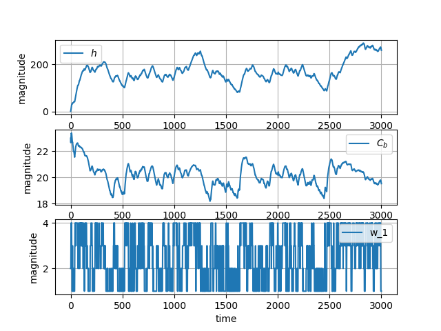
The input $w_1$ and the output $C_b$ save in arrays. The simulation have a duration of 3000 seconds. The initial values are $h(0) = 1$ and $C_t(0) = 23$ . Plotting the simulation have the next result

System with random input

The next step is the training. First prepare the data shifting one position the output array x to have the future values, so that lost a value therefore the training use 2999 data points.

# Prepare the data for training
datainp = np.append( x[:-1,1].reshape(n-1,1), np.array(u[:-1]).reshape(n-1,1) ,axis=1)
datatar = x[1:,1].reshape(n-1,1)

The datainp array have the input an the output in the present and the array datatar have the future value of the system. Then propose the ANN

# Set a ANN with two inputs, one hidden layer and one output layer
net = nl.net.newff([[0, 25], [0, 4]], [1, 1],[nl.trans.TanSig(),nl.trans.PureLin()])
 
# Set the initial value to the weights
net.layers[0].np['w'][:] = 0
net.layers[1].np['w'][:] = 0
net.layers[0].np['b'][:] = 1
net.layers[1].np['b'][:] = 1

Define the ANN with two inputs, two layers and the activation functions proposed. The initial values for the training are $w_1 = w_2 = w_3 = 0$ and $b_1 = b_2 = 0$ . Next have to train the ANN

# Change error function
net.error = nl.error.MAE
 
# Train network
num_epochs = 200
error = net.train(datainp, datatar, epochs=num_epochs, show=1, goal=0.1)
 
# Simulate network
out = net.sim(datainp)

Set the error function as MAE. Define the maximum number of epochs in 200 and the goal of the training as a 0.1. After the training proof the ANN with the same dataset. Plotting the error vs epochs have

Error through epochs

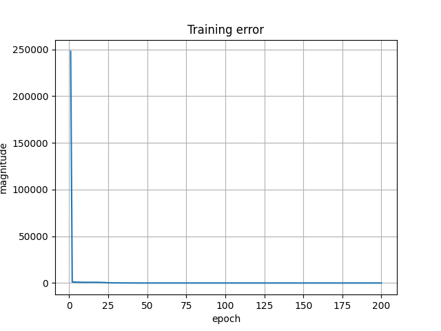
The error in the final epoch is around 0.9. Then plot the ANN prediction and the system output with the same random input

System and ANN

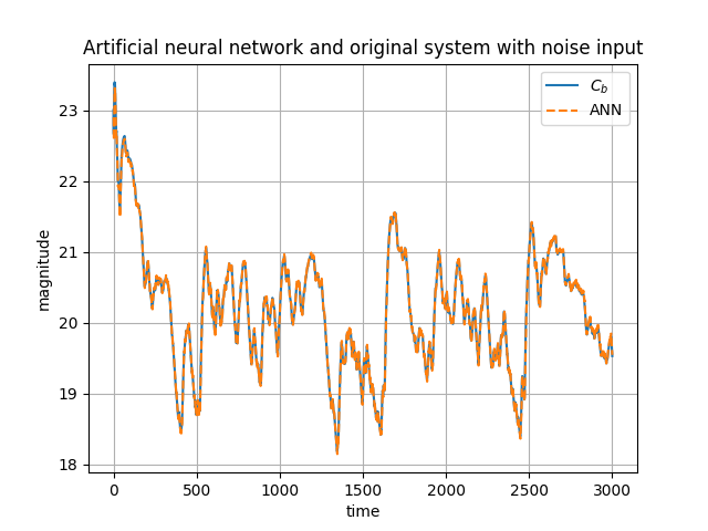
The ANN prediction is precise. The final weights values are $w_1 = 1.2482e-02$ , $w_2 = 2.5146e-04$ , $w_3 = 2.1492e+02$ , $b_1 = 0.831$ and $b_2 = -150.5797$ . Once the ANN predict the system the follow part is make the cost function minimization, for do that make a function

#Cost Function
def cost_fun_min(u,y,yn,ym,r,b,s,w1,w2,w3,b1,b2):
 
   com_arg = b1 + y*w1 + u*w2
   dyn_du = w3*w2*((1/(np.cosh(com_arg))**2))
   d2yn_du2 = -2*w3*(w2**2)*(np.tanh(com_arg))*((1/(np.cosh(com_arg)))**2)
   dJ_dU = -2*(ym - yn)*dyn_du - s/((u + r/2 - b)**2) + s/((r/2 + b - u)**2)
   d2J_dU2 = 2*((dyn_du**2) - d2yn_du2*(ym - yn)) + (2*s)/((u + r/2 - b)**3) + (2*s)/((r/2 + b - u)**3)
   u_next = u - dJ_dU/d2J_dU2
 
   if u_next < 0:
       u_next = 0*u_next
 
   return u_next

The function first calculated a common argument that have many functions, next the first derivative of $y_n$ w.r.t. $u$ , then the second derivative of $y_n$ w.r.t. $u$ , next the first derivative of $J$ w.r.t. $u$ , then the second derivative of $J$ w.r.t. $u$ , then calculated the next input with Newton-Raphson method finally only take the positives values input because the system doesn’t support negatives values because the state $\dot{h}$ have a square.

For the simulation of all NGPC first set the initial conditions, in code is

# Initial conditions
x0 = [1,1]
 
# Time vector
n = 10000
tf = 1000
t = np.linspace(0,tf,n)
 
# Reference for the system
ym = np.array(int(n/4)*[19] + int(n/4)*[20] + int(n/4)*[21] + int(n/4)*[20.5])
 
# Initial condition for the input
u = np.array([[0]])
 
# Vector to save the result
x = np.array([x0])
 
# Predict value
xp = np.array([[x0[1]]])

The total time of the simulation is 1000 seconds, the references are four constant values, each constant hold for a quarter of the time (250 seconds), the values are $Ref_1 = 19$ , $Ref_2 = 20$ , $Ref_3 = 21$ and $Ref_4 = 20.5$ . The initial values for the states are $h = C_b = 0$ . Also create a vector for save the values of the input of control u, the output of the system x and the predicted value for the ANN xp. To solve the system use again odeint of scipy as show in

for i in range(1,n):
   # Delay time
   t_delta = [t[i-1],t[i]]
 
   # Integrate one step
   xint = odeint(model,x[-1],t_delta,args=(u[-1,0],))
  
   # Predict the system with Neural Network
   yn = net.sim(np.array([[xint[1,1],u[-1,0]]]))
    # Calculating next input
   u_next = cost_fun_min(u[-1,0],xint[1,1],yn,ym[i-1],10,10,10e-20,w[0,0],w[0,1],w[0,2],b[0,0],b[0,1])
 
   # Save de result for the next step
   x = np.concatenate((x,np.array([xint[1]])),axis=0)
   u = np.concatenate((u,np.array(u_next)),axis=0)
   xp = np.concatenate((xp,np.array(yn)),axis=0)

For the simulation the constant values of cost function are $s = 10e-20$ , $b = 10$ and $r = 10$ . Plotting the output of the system $y$ and the reference $Ref$ have the follow graph

Reference vs system

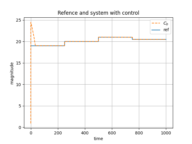
Other plot to see, is the comparison between the ANN prediction $y_n$ and the output of the system $y$

ANN vs system

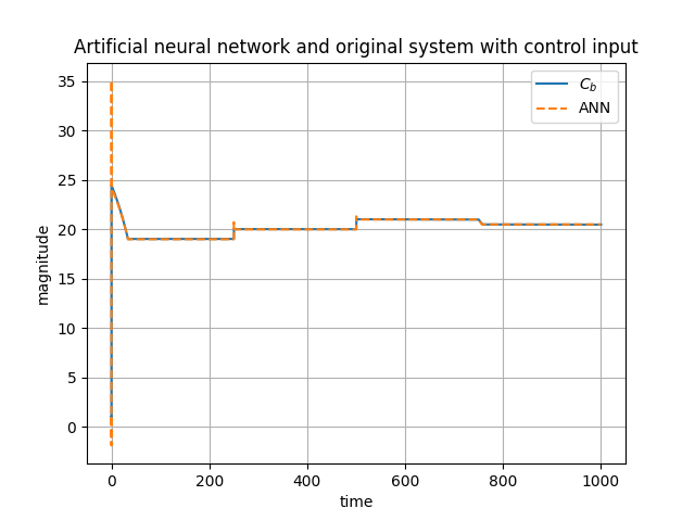
All the system with input control $u$ , the states $h$ and $C_b$ is showed in the next plot

System with NGPC

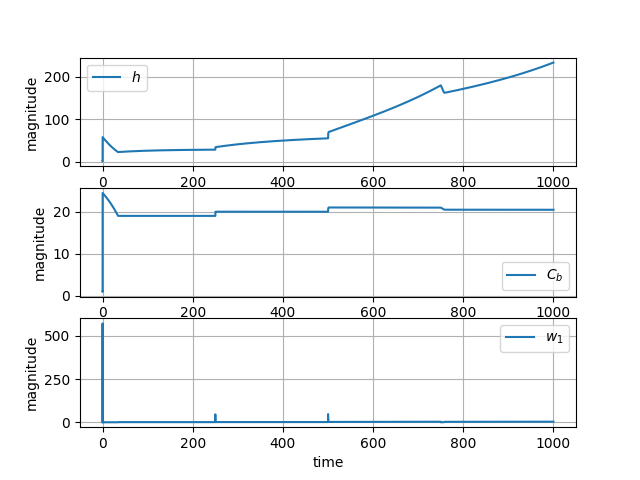
This is all the simulation

Conclusions and observations

The cost function:
- In the original paper in the cost function consider the change in the input $\Delta u$ . If cant affect the control input. For example in the beginning of the action control is a pick behold 500 this can change if consider the $\Delta u$ in the cost function.
The input and the system:
- The control input increase with the time, but if the input increase the state $h$ go to zero and uncontrollable. This is because the state $h$ are denominator in the part of the inputs of the state $C_b$ .
Comparison with MATLAB result:
- In parte this simulation is the same or trying to be the same as the example in MATLAB called design neural network predictive controller in simulink . The result aren’t the same. This can be because the cost function no are the same or in the MATLAB example use more than one future prediction and input.

References

All the references are linked in the text with underline and bold style, like this

Code

The complete code is in my GitHub